This is section 4 in my series on using Variational Inference to speed up relatively complex Bayesian models like Multilevel Regression and Poststratification without the approximation being of disastrously poor quality.
The general structure for this post and the ones after it will be to describe a problem with VI, and then describe how that problem can be fixed to some degree. Collectively, all the small improvements in these four posts will go a long way towards more robust variational inference. I’ll also have a grab bag at the end of other interesting ideas from the literature I think are cool, but maybe not as important or interesting to me as the 3 below.
In the last post we took a look at how our ELBO objective requires specific version of KL Divergence (the “Exclusive” formulation of KLD), and saw that it encoded a preference for a certain type of solution to the VI problem. Then we looked at CUBO and CHIVI, an alternative bound and algorithm that avoid this problem, often leading to a more useful posterior distribution by pursuing a more “inclusive” solution.
In this post, we’ll leverage importance sampling to make the most of the samples we do have, emphasizing the parts of our q(x) that look like p(x) and de-emphasizing the parts that do not.
The rough plan for the series is as follows:
Introducing the Problem- Why is VI useful, why VI can produce spherical cows
How far does iteration on classic VI algorithms like mean-field and full-rank get us?
Problem 1: KL-D prefers exclusive solutions; are there alternatives?
(This post) Problem 2: Not all VI samples are of equal utility; can we weight them cleverly?
Problem 3: How can we get deeply flexible variational approximations; are Normalizing Flows the answer?
Problem 4: How can we know when VI is wrong? Are there useful error bounds?
Better grounded diagnostics and workflow
Not all samples are equally good
So we’ve made an approximation q(x) that’s cheap to sample from, and is somewhat close to p(x), our true posterior. The way to improve the approximation we’ve focused on so far is to just go back to the start and make q(x) better; for example, through changing up the variational family, or to switching to a different optimization objective like the CUBO. That’s one solution that’s often necessary, but can we work with a particular q(x) we have and make better use of the parts of it that are the closest to being right?
… Phased this way, this sounds a lot like importance sampling. If you haven’t seen them before, an importance sampling estimator allows us to take draws from a (preferably) easy to sample from distribution1 and reweight the samples to look more like our true target distribution. The weight w_i (or ratio, r_i) for each sample i take form:
w_i = \frac{p(x_i)}{q(x_i)}
Before you get worried that we don’t have p(x_i) because of the normalizing constant like every time we talk about having p(x) in this series, there’s a clever estimator that “self-normalizes” such that this can be a reasonable strategy. Intuitively, we’re just placing more weight on samples more likely under p(x).
This footenote2 has a selection of some of my favorite resources for learning more or refreshing your memory about importance sampling, but for the main discussion let me pull out some particularly important sub-problems to solve in making a good importance sampling estimator, and good important sampling estimator for VI.
First, our choice of the “proposal” distribution we’re reweighting to be more like p(x) matters for making this process practically feasible. We need the proposal distribution to be close enough to p(x) that a realistic number of the draws get non-negligible weights. It might be true that we could draw proposals from a big N dimensional uniform distribution for every problem, but if we want to be done sampling enough this century we need to at least get fairly close with our initial q(x).
A second, but related problem is that it’s quite common for the unmodified importance sampling estimator to have some weights which are orders and orders of magnitude higher than the average weight, blowing up the variance of the estimator. Dan Simpson’s slides I linked above has an instructive example with not too weird p(x) and q(x)’s, but high dimension, that has a max weight ~1.4 million (!) times the average. If that happens, our estimator will essentially ignore most samples without gigantic weights, and it’ll take ages for that estimator to tell us anything remotely reliable.
So with those points we need to address, here are the next topics in this post:
Importance Weighted Variational Inference
Robust importance sampling with built in diagnostics via Pareto-Smoothed Importance Sampling
Combining multiple proposal distributions via Multiple Importance Sampling
Importance Weighted Variational Inference
Importance Weighting for VI in it’s simplest form is pretty intuitive (draw samples from an already trained q(x), weight them…), so let’s derive the new Importance Weighted Variational Inference (IWVI) estimator first since some nice intuition will come with it.
I want to emphasize something that wasn’t clear to me for a good while- these two ideas are not equivalent. While both are useful tools, the “train time”, objective-modifying IWVI estimator is a distinct approach from the “test time” importance sampling approach that takes draws from a fixed q(x) and reweights them as best it can.
We’ll aim to show that we can get a tighter ELBO by using importance sampling. This type of tighter ELBO was first shown by Burda et Al. (2015) in the context of Variational Autoencoders after which is was fairly clear this could apply to variational inference, but Domke and Sheldon (2018) fleshed out some details of that extension- I’ll be explaining some of the latter group’s main results first.
To start, imagine a random variable R, such that \mathbb{E}{R} = p(x), which we’ll think of as a estimator of p(x). Then by Jensen’s Inequality:
The first term is the bound, which will be tighter if R is highly concentrated.
This is a more general form of the ELBO; we can make it quite familiar looking by having our R above be:
R = \frac{p(z,x)}{q(z)}, z \sim q
The reason for pointing out this fairly simple generalization is helpful is that it frames how to tighten our ELBO on logp(x) via alternative estimators R.
By drawing M samples and averaging them as in importance sampling, we get:
R_M = \frac{1}{M}\sum_{m=1}^{M}\frac{p(z_m,x)}{q(z_m)}, z_m \sim q
From there, we can derive a tighter bound on logp(x), referred to as the IW-ELBO:
IW-ELBO_M[q(z)||p(z,x)] := \mathbb{E}_{q(z_{1:M})}log\frac{1}{M} \sum_{m=1}^{M}\frac{p(z_m,x)}{q(z_m)}
Where we’re using the 1:M as a shorthand for q(z_{1:M}) = q(z_1)...q(z_M).
It’s worth noting that the last few lines don’t specify a particular form of importance sampling- we’re getting the tighter theoretical bounding behavior from the averaging of samples from q. We’ll see a particularly good form of importance sampling with desirable practical properties in a moment.
How does IW-ELBO change the VI problem conceptually?
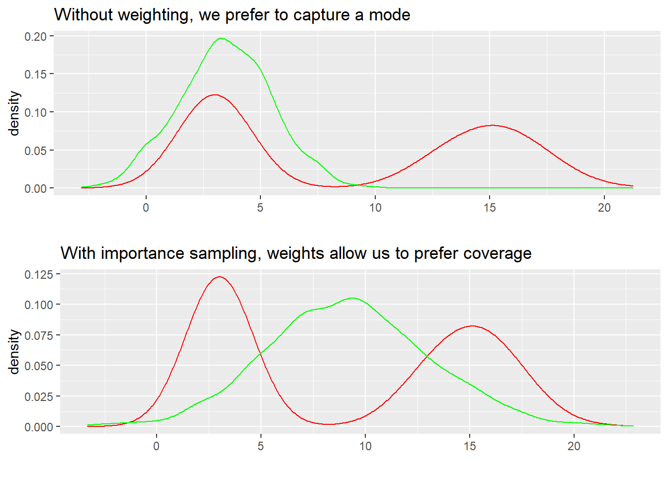
The tighter bound is nice, but importance sampling also has the side effect (done right, side benefit) of modifying our incentives in choosing a variational family. To see what I mean, we can re-use the example distributions from last post we used to build intuition for KL Divergence, where red was the true distribution, and green were our potential approximations. If we’re not going to draw multiple samples and weight them, it makes sense to choose something like the first plot below. Every draw in the middle of the two target modes is expensive per our ELBO objective, so better to choose a mode.
rkl_plot <- mixture %>%ggplot(aes(x = normals)) +geom_density(aes(x = normals), color ="red") +geom_density(aes(x = mode_seeking_kl), color ="green") +ggtitle("Without weighting, we prefer to capture a mode") +xlab("")fkl_plot <- mixture %>%ggplot(aes(x = normals)) +geom_density(aes(x = normals), color ="red") +geom_density(aes(x = mean_seeking_kl), color ="green") +ggtitle("With importance sampling, weights allow us to prefer coverage") +xlab("")grid.arrange(rkl_plot,fkl_plot)
If we can use importance sampling though, quite the opposite is be true! Note that we’re still using the ELBO, a reverse-KL based metric- that hasn’t changed. What has changed is our ability to mitigate the objective costs of those samples between the two extremes. Via this “train time” implementation of IS, points outside the two target modes will get lower importance weights, and points within the modes will get higher ones, so as long as we’re covering the modes with some reasonable amount of probability mass, and drawing enough samples we can actually do better with the distribution centered between the modes.
To further drive home the point about how a “train time” and “test time” implementations of IS differ, could “test time” IS do this? Not really- because the ability to better minimize the ELBO via sampling requires the IW-ELBO variant and associated training process. If we hard-coded q(x) as the green N(9,4) shown above, “test time” IS could weight the right samples up to better approximate p(x), but it doesn’t fundamentally alter our optimization problem the way the IWVI objective does.
We can also imagine how varying the number of samples might effect optimization. Between S=1 and “enough draws to get all the benefits of IS”, we can imagine there’s a slow transition from “just stick with 1 mode” and “go with IS”. So it seems like we should be worried about getting the number of samples right, but fortunately as we’ll see in the next section there are great rules of thumb in some variants of IS. We’ll still need to bear the cost of sampling (which gets higher as q(x) becomes “further” from p(x), as we’ll need more samples to weight into a good approximation), but the cost of sampling for most VI implementations will often be pretty manageable if our proposal distribution is somewhat close to p(x).
Another way to think about how importance sampling changes our task with variational inference is to think about what sorts of distributions make sense to have as our variational family, and even which objective might be better given IS. On choice of a variational family, if we’re aiming for coverage, moving towards thicker-tailed distributions like t distributions makes a lot of sense. While we explored the IW-ELBO above to build intuition, there’s no reason not to apply IW to the CUBO and thus CHIVI- this also naturally produces nicely overdispersed distributions which can be importance sampled closer to the true p(x). This idea of aiming for a wide proposal to sample from is referred to in the importance sampling literature (eg Owen, 2013) as “defensive sampling”, with Domke and Sheldon (2018) exploring the VI connection more fully. For intuition, by ensuring most of p(x) is covered by some reasonable mass makes it easier to efficiently get draws that can be weighted into a final posterior, even if the unweighted posterior might be too wide.
Solving our IS problems with Pareto-Smoothed Importance Sampling
As we’ve been talking about importance sampling, we’ve been leaving some of the messier details aside (how many samples to draw, how to deal with the cases when some of the weights get huge, how to know when our proposal distribution is “close” enough).
While the Importance Sampling Literature is huge and there are a lot of possible solutions here, I’ll next introduce Vehtari et Al. (2015)’s Pareto-Smoothed Importance Sampling. I’m a huge fan of this paper- it’s a really elegant and powerful tool, derived from taking Bayesian principles seriously.
Above, I described a common failure mode for IS estimators, where some weights are orders of magnitude larger than others, with this long right tail of ratios dominating the weighted average and blowing up the variance of the estimator. Pareto-Smoothed Importance Sampling proposes to model those tail values as coming from a Generalized Pareto Distribution, a distribution for describing extreme values, and replace the most extreme weights with modeled (and more stable) values.
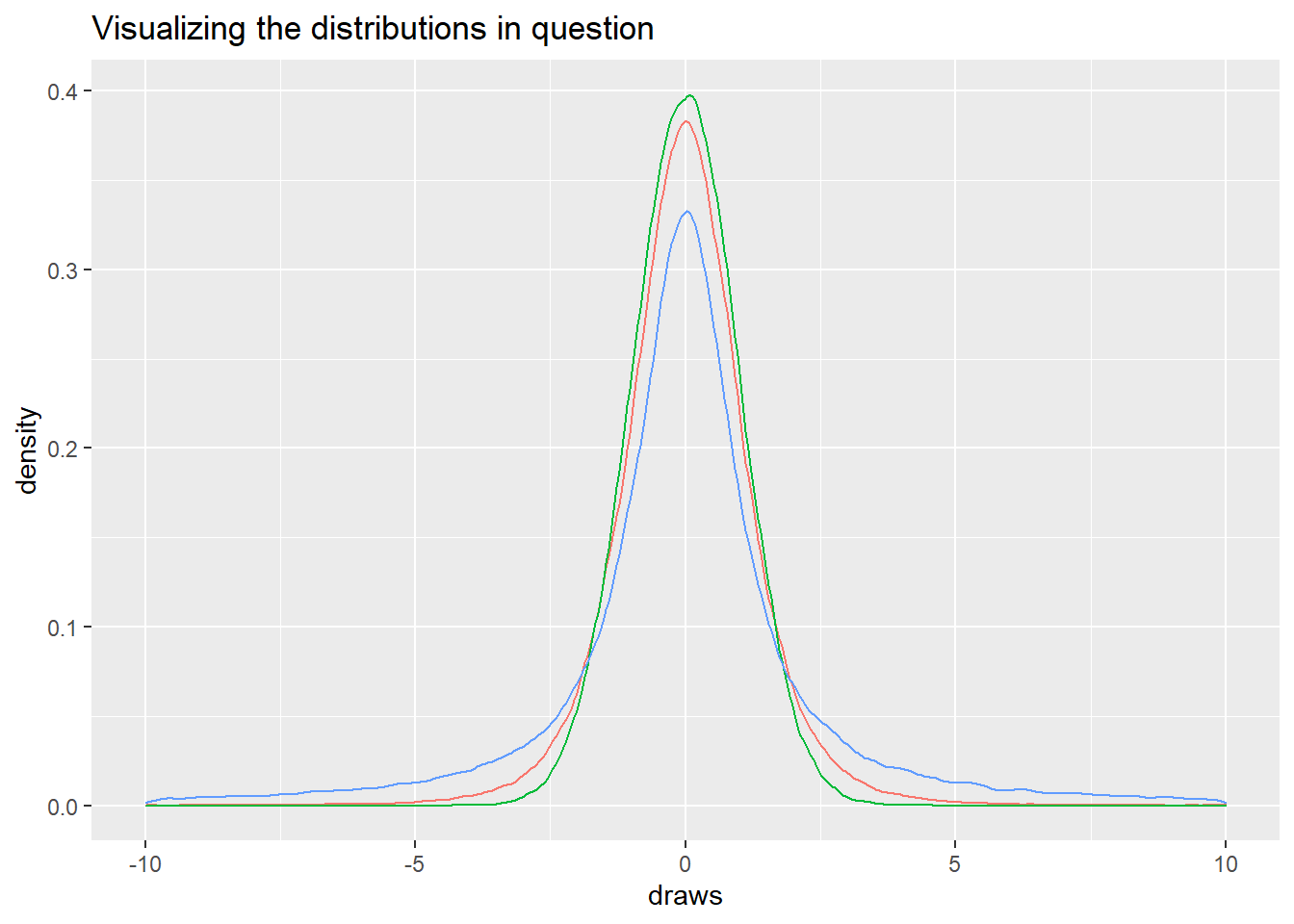
For concreteness, let’s introduce a simple 1-D example. We’ll aim to use importance sampling to approximate distributions \mathcal{T}(\mu = 0,\sigma = 1,t =5) and \mathcal{C}(x_0= 0,\gamma = 10) with a \mathcal{N}(\mu = 0,\sigma = 1) distribution. If that sounds like the opposite of preferring wide tails on q(x)’s I described above, you’re right, but using a poor choice here will illustrate some useful properties.
simulated_data <-tibble(q_x =rnorm(100000),manageable_p_x =rt(100000,5),unmanageable_p_x =rcauchy(100000),manageable_ratios =dt(q_x,5)/dnorm(q_x),unmanageable_ratios =dcauchy(q_x,0,10)/dnorm(q_x))simulated_data %>%pivot_longer(c(q_x,manageable_p_x,unmanageable_p_x),values_to ="draws",names_to ="distributions") %>%ggplot(aes(x = draws, color = distributions)) +geom_density() +# If you wanted to show the full reach of the Cauchy, it'd be# hard to see the shape of the T vs N; it's that wide.# Hence the 6k values removedxlim(-10,10) +ggtitle("Visualizing the distributions in question") +theme(legend.position="none")
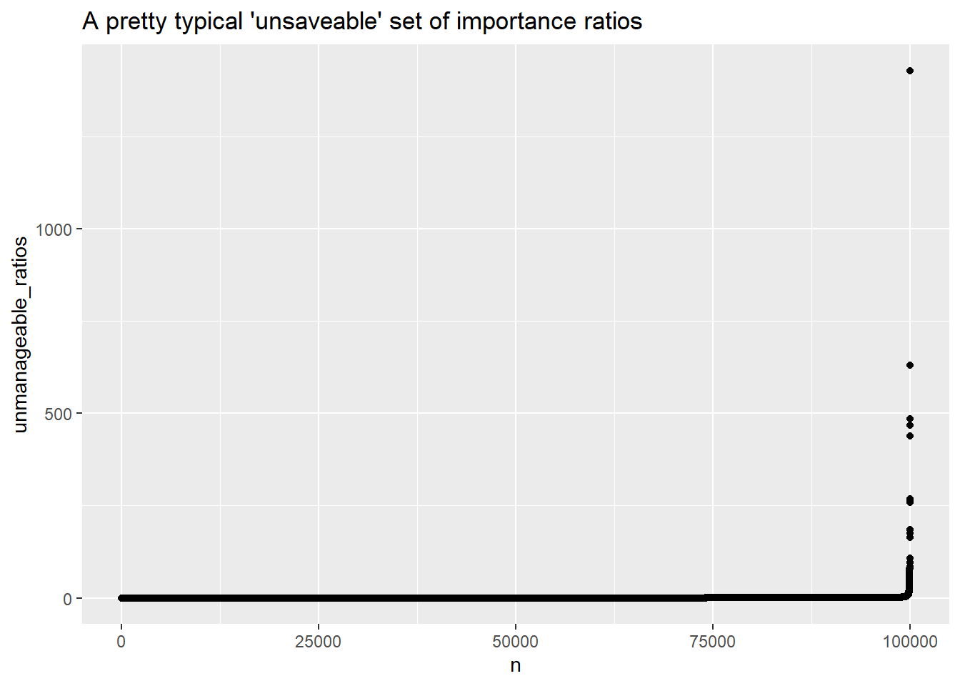
The tails on that Cauchy distribution are super, super wide compared to our normal, so the samples far, far out in the tails of the normal will need massive weights to approximate the cauchy. The t-distribution is wider too, so we’ll need some higher weights, but not nearly as many. As a way to visualize this, you can see that just a handful of draws have weights away from ~1, but these weights are as much as 5000x higher than the mean ratio, and will dominate any average we make of them.
simulated_data %>%arrange(unmanageable_ratios) %>%mutate(n =seq(1,100000)) %>%ggplot(aes(x = n,y = unmanageable_ratios)) +geom_point() +ggtitle("A pretty typical 'unsaveable' set of importance ratios")
The t-distribution ratio plot would look similar, but with a much smaller y-scale. The max weight would still be much larger than the average, but more than an order of magnitude or so less large:
mean_t <-mean(simulated_data$manageable_ratios)max_t <-max(simulated_data$manageable_ratios)mean_c <-mean(simulated_data$unmanageable_ratios)max_c <-max(simulated_data$unmanageable_ratios)print(paste0("the mean of the t is: ",mean_t," compared to a max of ",max_t,";","The cauchy cause is more extreme- the mean of the cauchy is: ",mean_c," compared to a max of ",max_c))
[1] "the mean of the t is: 0.995904306317625 compared to a max of 164.448932152079;The cauchy cause is more extreme- the mean of the cauchy is: 0.283655933763642 compared to a max of 1428.22324178729"
So let’s bring this back to Pareto smoothing here. We want to model and smooth that long tail of the ratio distribution. It turns out there’s plenty of study of the distribution of extreme events, and there’s some classical limit results showing:
where \tau is a lower bound parameter, which in our case defines how many ratios from the tail we’ll actually model. \sigma is a scale parameter, and k is a unconstrained shape parameter. Without getting too far into the weeds, we can implicitly define \tau via using a well-supported role of thumb suggesting to use the M largest ratios, M = min(0.2S,3\sqrt{S})3. From there, the \hat{k} and \hat{\sigma} have easy and efficient estimators. The Generalized Pareto Distribution has form:
and we can replace our M biggest ratios with estimated values calculated via the CDF of the Generalized Pareto Distribution.
One of the best things about PSIS is it comes with a built in diagnostic via \hat{k}. To see how this works, it’s useful to know that importance sampling depends on how many moments r(\theta) has- for example, if at least two moments exist, the vanilla IS estimator has finite variance (which is obviously required, but no guarantee of performance since it might be finite but massive). The GPD has k^{-1} finite fractional moments when k > 0.
Vehtari et al. show that the replacement of the largest M ratios above changes PSIS to have finite variance and an error distribution converging to normal when k \in (.5,1). Intuitively, k > .5 implies the raw ratios have infinite variance, but PSIS trades a little bias to make the variance finite again.
What about actually practical to work with variance? This is the really cool bit- k < .7 turns out to be a remarkably robust indicator of when we can expect PSIS to work in a ton of different simulation studies and practical examples.
Why is this true? 1.4 fractional moments seems awful arbitrary, right? Let’s ask an alternative question, and kill two birds with one stone: what sample size do we need for PSIS to work? Chaterjee and Draconis (2018) showed that for a given accuracy, how big S needs to be for importance sampling more broadly depends on how close q(x) is to p(x) in KL distance- we need to satisfy log(S) \geq \mathbb{E}_{\theta \sim q(x)}[r(\theta)log(r(\theta))] to get accuracy.
Well, we don’t know the distribution of r, we should have some pretty good intuition that the important part (read: that explosive, variance ruining tail) is Pareto. If we take r as exactly Pareto, you can trace out S for different \hat{k}4, and to give a few example points-
for given \hat{k}, roughly what S is needed if r is exactly Pareto
\hat{k}
S needed
.5
~1,000
.7
~140,000
.8
1,000,000,000,000
.9
please stop you’re making your compute sad.
While we of course know r isn’t Pareto exactly exactly, hopefully this helps with intuition around \hat{k} telling us when we’re getting into “sampling forever to have any chance at all to control the variance” land.
Neat! So what does that look like for our Cauchy and T distribution example?
As we expected, the the Normal proposal distribution isn’t ideal for the T distribution, but it’s manageable. On the other hand, we’d need somewhere between a trillion and “oh god no :(” samples to make the normal proposal work out for the Cauchy.
Bringing the discussion back to variational inference, PSIS is super helpful- importance sampling more generally broadens the class of q(x)es that are close enough to p(x) for variational inference to work, and PSIS considerably widens that basin of feasibility. The extensive theoretical and simulation framework around the method also give us a solid way to realize when importance sampling isn’t feasible via the \hat{k} diagnostic, and tells us how roughly samples we need to draw. Super, super cool.
One more great thing PSIS does for variational inference- \hat{k} serves as a powerful diagnostic for variational inference itself! I’ll save most of this discussion for the post on diagnostics, but to sketch out the logic- \hat{k} tells us when q(x) is too far from p(x) for importance sampling to work, which is a function of KL Divergence from q(x) to p(x)- if that distance is too great for importance sampling to allow us to bridge, that implies we aren’t close enough to trust our base variational approximation either!
Multiple Proposal Distributions with Multiple Importance Sampling
Why stop at just one proposal distribution? This is basically the jumping off point for Multiple Importance sampling, or MIS. If we have several different q(x), and each does a somewhat better job of handling a certain region of the target posterior, then we can efficiently combine them using MIS into an overall better final estimate, and this will work out to be pretty obviously more optimal than just fitting a bunch of VI approximations and averaging them.
If we can suddenly have multiple different q(x) working together, this naturally explodes the search space for a good VI strategy. I’d refer the more interested reader to Elvira et al. (2019) which lays out a framework for thinking about all the decision space of MIS more comprehensively, but for the purposes of improving VI specifically, I’ll cover:
How do we weight the proposals together?
Which proposals make sense to include in a MIS framework?
How practical is fitting multiple proposals?
How do MIS weights work?
How do we generalize a notion of importance weights like the one introduced above:
w_i = \frac{p(x_i)}{q(x_i)}
to multiple proposals? While there are some obviously not good properties we want to avoid (it’d be pretty silly to give up our unbiasedness), there are a ton of apparent degrees of freedom in MIS weighting. we’ll relax this assumption in a bit, but let’s start by assuming we don’t have any prior information about which proposals might be better, and that we’ll draw the same number of samples from each proposal.
While I won’t work through as extensive of an example as in the last section, let’s fix an example where we’ll have J = 3 different proposals, q_1(x)), q_2(x), and q_3(x)).
A first question is how to choose the denominator in the weight. One simple and efficient option is to simply use the density of a sample from j to make a weight, for example weighting a draw from q_3(x)) as:
w_{i} = \frac{p(x_i)}{\textcolor{pink}{q_3(x_i)}}
This works, and is pretty common in MIS applications, but we’re not really using all the information we have from having several proposals. We can get a provably lower variance estimator by defining the mixture of the densities \psi(x) as:
and using that as the denominator. So for the example above, this’d be:
w_{i} = \frac{p(x_i)}{\frac{1}{3}(\textcolor{cyan}{q_1(x)} + \textcolor{purple}{q_2(x_i)} + \textcolor{pink}{q_3(x_i))}}
By defining this mixture and and incorporating it into our weighting, we intuitively should have more efficient exchange of information between the different q(x). By this, I mean that we no longer just are weighting each sample from a proposal using information from that one proposal; we’re now using everything at hand.
This feels like it should be pretty solidly better than just using a single proposal density, and indeed Elvira et al. have a result showing that the variance of the mixture based weighting scheme is under pretty general conditions lesser than or equal to that of the single proposal density one5.
Veach and Guibas (1995), the paper to introduce MIS, called this weighting scheme the balance heuristic, since the weighting scheme is unique in that each sample value at particular x is the same regardless of which distribution produced it. They also prove a bound on the variance of this estimator, showing that there isn’t a lot of room to improve on it, even in the most ideal circumstances. Without getting into the weeds, their result suggests that there isn’t a massively better general-case weighting scheme, which is a helpful guide to practical use.
When can we do (a bit) better than the weighting scheme above? The answer is essentially in cases where we know some of our J proposals are much better than others. In these situations, the variance can often be lowered by pushing weights towards the extremes, making low weights closer to zero, and high weights closer to 1. Their cutoff heuristic suggests an estimator where you pick some bound \alpha, below which low weights are reassigned to zero (and the rest of the distribution is adjusted back to sum correctly). Their also propose the power heuristic-
w_i = \frac{p_i^\beta}{\sum\limits_{j}p_j^\beta}
which raises the weights to a power \beta, and normalizes. For intuition, notice that if \beta = 1, then this is the balance heuristic again, and as \beta \rightarrow \infty, this moves towards only selecting the best proposal at each point.
As a final note, we can also Pareto Smooth any of these types of weights once we have them, and this sparks joy, as we can add begin to envision model setups with glorious abbreviations like IW-ELBO/IW-CUBO-PSIS-MIS-VI.
So stepping back, we have some provably efficient, provably hard to beat ways to use MIS to combine variational approximations together. Again, there’s a whole literature on MIS which the Elvira paper above reviews, but fairly intuitive weighting schemes exist that work well in most cases, and there are reasonable things to try in more atypical cases to reduce the variance of the MIS estimator as well.
What proposals combine best?
A next natural question is what different proposals should we use? There’s a little less work in this area than I expected, but there are a couple of papers; my favorite is Lopez et al. (2020)6.
They find that using VI approximations based on different objectives is quite performant- for example, having all of a vanilla ELBO, IW-ELBO and \chi^2 divergence based VI approximation works particularly well, and as you’d expect, better than any individual model, just like we’d expect with regular ensembling techniques. They also look at taking some samples directly from our priors, which is moderately surprising to me given how broad weakly-informative priors usually are. Overall though, a core nugget of logic from ensembling more generally applies here too: we want to find proposals that are both good and sufficiently different from one another that combining them adds value.
It seems to me there’s a lot of room to explore this search space still; there are a lot of generic ML ensembling tricks that feel like they could work. For example, could we save state several times throughout optimizing a variational approximation, and MIS combine samples from each of those, similar to how people cheaply ensemble for neural networks? Or are there ways to optimize the proposals for use together in this way?
How practical is MIS for VI?
A last obvious question is whether fitting many variational approximations and combining them is computationally practical. While MIS for VIS certainly trades back some computational cost and time for potential accuracy, the good news is everything feels cheap compared to MCMC.
Fitting J VI approximations instead of 1 roughly scales your compute need for fitting the models by a factor of ~J, and then there’s a small additional cost in the MIS combination stage to evaluate all the models to make each importance sampling weight denominator. Unlike with MCMC, these computational needs are parallelizable.
Lopez et al. (2020) find that using 3 proposals slightly more than triples their compute cost given all the objective based models take around the same time to fit, and in practice slightly more than triples their compute time as well since they didn’t do the work to parallelize their models. On the problems they were working on, this is a pretty small (~30s more) time cost in exchange for a meaningful accuracy improvement in the real world biology application they apply this to.
Depending on what you’re working on, the answer may well be yes, this can be computationally feasible and well worth it.
Conclusions
Importance Sampling is a workhorse of modern computational statistics, and it should be no surprise it brings a lot to variational inference.
Like with the last post, my overall impression is of decreasing fragility for variational inference and a broader set of tools for increasing performance. With IW-ELBO and similar objectives, we can get a tighter bound than the vanilla ELBO, and introduce some new incentives in training our approximation as well. With importance sampling in general and PSIS especially, we can weight an approximation that is close to the target but not perfect into a much, much better approximation of our posterior, and do some in a principled and theoretically grounded way with built-in diagnostics. With MIS, we can make the most of several approximations at once, if we’re willing to pay that computational cost. Collectively, we’re building up a set of tools that broaden the class of problems for which VI works, provided you’re willing to spend time searching for a combination of tools that works well for your specific application.
Thanks for reading. In the next post, we’ll look at Normalizing Flows, an incredibly powerful and general tool for making maximally flexible variational distributions. All code for this post can be found here.
Footnotes
we’ll call it q(x) here to make the application super clear, but often I see the “proposal” distribution called g(x) and the the distribution we want to approximate called p(x). Another common notation would be \pi(x) for the target and q(x) for the proposal. It’s also helpful to know that the computer graphics (as in, image rendering) community is the source of a lot of work especially around Multiple Importance Sampling since they need to solve lots of light transport integrals, and they have yet another set of conventions from most statisticians, but you can usually figure out their choices by squinting a bit.↩︎
If you’re looking to learn about importance sampling for the first time, a great place to start is Ben Lambert’s video introductions to the basic idea: video 1, and video 2. For building more intuition about why we need all these variance reducing modifications to general IS, Dan Simpson has some great slides which have a side benefit of being hilarious. Those slides will mention a lot of the books/papers I find most instructive, but it’s worth calling out especially Vehtari et Al’s Pareto Smoothed Importance Sampling paper as particularly well written and paradigm shaping. Finally, Elvira et Al’s (2019) Multiple Importance Sampling paper is the most thorough I know, but isn’t particularly approachable. Instead, for MIS I’d recommend starting with the first few minutes of this talk (although the main topic of their talk is less relevant, the visualizations are super helpful), and the first ~8 pages of this paper, also by Elvira et Al. (2021) (I especially like that it spends a bit more time on notation; since multiple importance sampling comes from/comes up in computer graphics, the notational choices sometimes feel a bit annoying to me). Finally, the original MIS paper itself, Veach & Guibas (1995) is quite readable, but requires a bit of reading around or reading into computer graphics to grok their examples and notational choices.↩︎
Slight more weeds here- it turns out that this idea to use Vehtari et al.’s rule of thumb for selecting M and getting \tau from there is fairly important. The GPD Approximation is pretty sensitive to getting \tau right- it’ll be poor if \tau is too low. Having a deterministic rule of thumb that preforms better than alternative more complicated schemes for estimating \tau is great, and they work through showing it works well in most reasonable cases.↩︎
I’ll be lazy here and not derive or plot this- you can see the plot in Dan Simpson’s slides mentioned above.↩︎
One fascinating caveat here is that they proved this only for the case where we know the normalizing constant, not the self-normalized case we pretty much always have to live with, but they have some numerical results and some pretty common sense arguments that the result should extend in most reasonable cases to SNIS as well.↩︎
Worth noting that one of the authors here is Michael l. Jordan, which is a pretty good heuristic for “this will be a banger of a stats paper”.↩︎